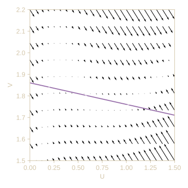
We do the thing we keep doing this course:
$$\begin{aligned}
\frac{dP_i}{dt} = \underbrace{d_P\left( P_{i-1}+P_{i+1} \right)}_{\text{hopping to i}}-\underbrace{2d_PP_i}_{\text{hopping away}}+\underbrace{\alpha(P_i,F_i)P_iF_i}_{\text{plant duplicates}}-\underbrace{\beta(P_i,F_i) P_i}_{\text{plant dies}}\\
\frac{dF_i}{dt} = \underbrace{d_F\left( F_{i-1}+F_{i+1} \right)}_{\text{hopping to i}}-\underbrace{2d_FF_i}_{\text{hopping away}}-\underbrace{\alpha(P_i,F_i)P_iF_i}_{\text{food eaten}}+\underbrace{\beta(P_i,F_i) P_i}_{\text{new food}}
\end{aligned}$$
Reaction Diffusion Equations
Taking the continuum limit, we get:
$$\begin{aligned}
P_t = D_P P_{xx}+\alpha(P,F)PF-\beta(P,F) P\\
F_t = D_F F_{xx}-\alpha(P,F)PF+\beta(P,F) P
\end{aligned}$$
for example: we can pick $\alpha(P,F)=1$ and $\beta(P,F) = \frac{1}{1+P}$.
So constant absorbtion
rate of nutrients, and plants die less and less when there's more of them.
Same choice as "Phase-separation physics underlies new theory for the resilience of patchy ecosystems" by Koen Siteur et al. (2022)
More generally, with a bit of rescaling, we get:
$$\begin{aligned}
U_t&=\epsilon^2 U_{xx}+f(U,V)\\
V_t &=V_{xx}-f(U,V)
\end{aligned}$$
with $f$ now a general function of $U$ and $V$, now some generalized concentrations.
(Big)
simplification for analysis: $\epsilon\ll1$.
My thesis - Existence
First question: Are there (localized) patterned solutions $(\bar U(x),\bar V(x))$?
Answer: Yes, under certain conditions on $f(U,V)$, we get "front" solutions, with two "plateaus" and
a transition part.
My thesis - Stability
Second question: Are those fronts stable? $(\bar U(x)+\delta u(x,t),\bar V(x)+\delta v(x,t))$
Answer (work in progress): Yes, when both the plateaus are stable, so is the complete front.
My thesis - Interaction
Third question: How do the fronts interact?
Answer (work in progress): Exponentially slow, so most likely not super relevant in actual systems.
My thesis - Higher Dimensions
Fourth question: Can we extend to 2 dimensions?
Answer (guessing): In similar systems, something like surface tension happens.
Questions?
Steady state
$$
\begin{aligned}
U_t &= \epsilon^2 U_{xx}+f(U,V)\\
V_t &= V_{xx}-f(U,V)\\
\end{aligned}
$$
In steady state:
$$
\begin{aligned}
0 &= \epsilon^2 U_{xx}+V_{xx}\\
\end{aligned}
$$
So: $V = \eta_0-\epsilon^2U$ in steady state ($\eta_0$ is constant of integration). Then:
$$
0=\epsilon^2U_{xx}+f(U,\eta_0-\epsilon^2U):=\epsilon^2U_{xx}+g_{\eta_0}(U)
$$
So a Hamiltonian system in $U$.
Existence of fronts
When do we get front solutions? Heteroclinics of $\epsilon^2U_{xx}+g_{\eta_0}(U)=0$. Writing $F'_{\eta_0}(U)=\epsilon^{-2} g_{\eta_0}(U)$ we get the Hamiltonian form:
$$
\frac12 (U_x)^2+F_{\eta_0}(U(x))=E\quad\forall x\\
$$
Now $F_{\eta_0}(U)$ plays the role of a potential in classical mechanics terms. If we can find an $E$ and $U_+\not =U_-$ such that $F_{\eta_0}(U_+)=F_{\eta_0}(U_-)=E$, $F_U(U_+)=F_U(U_-)=0$ and $F_{\eta_0}((U_-,U_+))\subseteq [L,E)$ for some $L$ smaller than $E$, we can expect a front solution.
Linearizing
When we have a steady state front: $(\bar U,\bar V)$, we can linearize around it to find its stability. Write:
$$
U = \bar U+\delta\exp(\lambda t)u+O(\delta^2),\,\,V = \bar V+\delta\exp(\lambda t)v +O(\delta^2)
$$
We find to leading order (in $\delta$) the steady state equations:
$$
\begin{aligned}
0 &= \epsilon^2 \bar U_{xx}+f(\bar U,\bar V)\\
0 &=\bar V_{xx}-f(\bar U,\bar V)\\
\end{aligned}
$$
And the next order equations read:
$$
\begin{aligned}
\lambda u &= \epsilon^2 u_{xx}+f_U(\bar U,\bar V)u+f_V(\bar U,\bar V)v\\
\lambda v &= v_{xx}-f_U(\bar U,\bar V)u-f_V(\bar U,\bar V)v\\
\end{aligned}
$$
Scales
We split space into two outer layers and one boundary layer: $I_f=[-\sqrt{\epsilon},\sqrt{\epsilon}]$, fast variable $\xi = x/\epsilon$, then in the fast coordinate, the boundary layer is $[-1/\sqrt\epsilon,1/\sqrt\epsilon]$, so in the limit of $\epsilon\to0$, this becomes the whole line.
Fast linearized
Introduce a fast variable $x=\epsilon\xi$:
$$
\begin{aligned}
\lambda u &= u_{\xi\xi} + f_U(\bar U,\bar V)u+\epsilon^2f_V(\bar U,\bar V)v\\
\epsilon^2\lambda v &= v_{\xi\xi} - \epsilon^2f_U(\bar U,\bar V)u-\epsilon^2f_V(\bar U,\bar V)v
\end{aligned}
$$
So we find that $v = v_0+\epsilon^2v_2$, we can use this to find:
$$
\lambda u = u_{\xi\xi} + f_U(\bar U,\bar V)u+\epsilon^2f_V(\bar U,\bar V)v_0
$$
An inhomogeneous Sturm-Liouville problem:
$$
u = (\mathcal L-\lambda)^{-1}v_0
$$
With $\mathcal L = \partial_{\xi\xi}+f_U(\bar U,\bar V)$. Since $\mathcal L$ is the operator corresponding to a heteroclinic with translational symmetry, it has an eigenvalue zero corresponding to shifts, so $\mathcal L \bar U_{\xi}=0$, but $U_\xi$ has strictly one sign, so $0$ is the largest eigenvalue of $\mathcal L$. So for growing modes ($\lambda>0$), this defines $u$.
Slow systems around boundary
In the slow subsystems, to leading order (here $\bar U,\bar V$ are constant):
$$
\begin{aligned}
\lambda u&=f_U(\bar U,\bar V)u+f_V(\bar U,\bar V)v\\
\lambda v &= v_{xx} -f_U(\bar U,\bar V)u-f_V(\bar U,\bar V)v\\
\end{aligned}
$$
denote $f_{U,l},f_{V,l}$ as the derivatives on the left side and similarly the right side are $f_{U,r},f_{V,r}$. Here, $u$ is determined in terms of $v$, so we can do a bit of calculus and find that at $\xi=\pm 1/\sqrt\epsilon$, we have:
$$
v_{\xi}(\pm1/\sqrt\epsilon)=\mp\epsilon \sqrt{\lambda +\frac{\lambda f_{V,r/l}}{\lambda-f_{U,r/l}}}+O(\epsilon^{5/2})
$$
Some algebra shows that $\epsilon^2\int_{-1/\sqrt\epsilon}^{1/\sqrt\epsilon}\lambda d\xi=2\epsilon^{3/2}\lambda$ cannot match the order of the slow timescale so we put those away in the higher order terms.
$$
\int_{-1/\sqrt\epsilon}^{1/\sqrt\epsilon}[f_U(\bar U,\bar V)u_{inner}+f_V(\bar U,\bar V)]d\xi= -\frac{\sqrt\lambda}{\epsilon}\left(\sqrt{1-\frac{f_{V,r}}{f_{U,r}}}+\sqrt{1-\frac{f_{V,l}}{f_{U,l}}}\right)
$$
Integral should have a real value. Then the left hand side should be real too. Then for positive, real $\lambda$, we require that the square roots be real. If they aren't, we can't have positive, real $\lambda$, which is interesting. This implies:
$$
f_{V,r}\leq f_{U,r},\quad f_{V,l}\leq f_{U,l}
$$
is necessary for instability in the form of a real (non-oscillating) eigenvalue.
Fourier - decoupling the waves
Let's check the stability around $(U_+,V_+)$. We linearize again:
$$
\begin{aligned}
u_t &= \epsilon^2 u_{xx}+f_U(U_+,V_+)u+f_V(U_+,V_+)v\\
v_t &= v_{xx}-f_U(U_+,V_+)u-f_V(U_+,V_+)v
\end{aligned}
$$
A quick Fourier transform (we assume we're far away enough from any structure that we can do this, other words, the slow reduced system), shows us that:
$$\begin{aligned}
\hat{u}_t = \epsilon^2(ik)^2\hat{u}+f_U \hat{u}+f_V\hat{v}\\
\hat{v}_t = (ik)^2\hat{v}-f_U\hat{u}-f_V\hat{v}
\end{aligned}
$$
We now write this as:
$$
\begin{pmatrix}\hat{u}\\\hat{v}\end{pmatrix}_t=
\begin{pmatrix}f_U-\epsilon^2k^2&f_V\\-f_U&-f_V-k^2\end{pmatrix}
\begin{pmatrix}\hat{u}\\\hat{v}\end{pmatrix}
$$
Fourier - trace and determinant
We get the determinant:
$$\begin{aligned}
\Delta\begin{pmatrix}f_U-\epsilon^2k^2&f_V\\-f_U&-f_V-k^2\end{pmatrix} &=(f_U-\epsilon^2k^2)(-f_V-k^2)+f_Uf_V \\
&= -f_Uk^2+\epsilon^2 k^2 f_V+ \epsilon^2k^4\\
&= k^2(\epsilon^2 k^2+\epsilon^2 f_V-f_U)
\end{aligned}$$
For stability of all wavenumbers, we need $\epsilon^2 f_V-f_U>0$. Next, we look at the trace, and find that
$$
\operatorname{Tr}\begin{pmatrix}f_U-\epsilon^2k^2&f_V\\-f_U&-f_V-k^2\end{pmatrix} =f_U-\epsilon^2k^2-f_V-k^2
$$
For stability, we require $\operatorname{Tr}<0$, so here we get another inequality for stability:
$$
f_V-f_U>0
$$
Leading order $\lambda$?
So the stability criterion of the plateaus tells us that $\lambda$ needs to be negative if it's real to leading order. Hence, if we can show that $\lambda$ equals the slow subsystems lambda to leading order, we're done.